Tune diagram in python

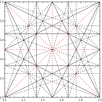
Resonance line diagram in python.

I am trying to move whatever I can to python. The main reason being that I want it to be free, and not require expensive commercial software. So recently I took the time to revisit my Mathematica code for the tune diagram and port it to Python. Basically I rewrote the whole thing and it has the nice feature that you can overlay it on top of whatever you want to plot.here you find my python code for plotting a resonance line diagram as the one found above.

The code should be self-explanatory, when you run the script directly with the option -o shows an example plot. When you import it, you can use the function plotTuneDiagram(maxOrder,xlim=[0,1],ylim=[0,1],tickOrders=False,tuneLineColor="black")

Parameters are

  • maxOrder the maximum order of resonance line to be displayed
  • xlim,ylim the intervals in horizontal and vertical tune in which to plot
  • tickOrders whether or not to place x- and y labels on full fractions up to selected order
  • tuneLineColor color for the tune lines, sensible when plotting on top of measurement or simulation data.

Server setup 1 (seafile vs OwnCloud)

Notice (27. Feb 2014): If you came here searching for „seafile lighttpd“: I wrote a comment on how to get it running on here, this article is only on my perceptions of seafile vs OwnCloud.

In the aftermath of the revelations about NSA spying, a few friends and I decided to buy a hardware (as opposed to virtual) root server together. We wanted to have a more private replacement for the majority of cloud services, most notably e-mail, Dropbox, rss reader and backup solutions.

Before getting the server I used a paid Dropbox account so for me moving away from paying Dropbox I would automatically save money to pay the server cost from. I needed paid because I kept around 30 gigagbytes of stuff on the Dropbox. My main requirement was to have a replacement that can handle large directories with tens of thousands of small files smoothly. I looked into two solutions:

OwnCloud

I tried Owncloud, first in a virtualbox ubuntu on my local box. There it was rather ok, working with Dropbox-like performance. During the setup of the server I ran a copy on remotely and tested it with the contents of my Dropbox. I have a few sourcecode folders in there, which, including their git repositories amount to about 100k files, most of them very small. Over the internet, Owncloud was really slow. Analogue modem-like slow. In the end the transfer speeds were below 10kb per second. Really not what you want your 30gig full dropbox folder to sync with. The test folder of a few gigabyte (around 2) was still syncing after one day on a 10mbit connection. So it is not a problem of „getting up to speed“. The reason for this seems to be that Owncloud (currently) uses one request per file. And maybe these are not even parallelized, adding a lot of delay to the file transfers.

seafile

Seafile follows a different concept from most of the other selfhosted cloud storage solutions. Instead of a file-based system it uses a revision-based approach based on a modified version of git. If you know the github interface, you know the seafile (web-) interface. For seafile the test with the 100k file folder managed to max out my connection bandwidth. For me this clearly indicated seafile as the preferrable solution and it is what we are now running for „production“. I deployed it with lighttpd and wrote a short post on the seafile mailing list here.

Another plus of seafile is that it supports client-side encryption. This makes it interesting even for people who want to run it on untrusted hardware or on a hosted solution. The server never sees the plain text data after all.

Platform independent, crude timing of code

I work a lot on MacOS where I write code that I want to use on linux later. Unfortunately some of the normal timing functions are missing on MacOS. I don’t quite remember which. So I have some crude platform independent code for timing c++ code. I am aware it does not really count the CPU usage, but putting it around code you want to time you can still get a feeling for how much time is spent in that part of your code.


class pTimer {
 timeval t1, t2;

public:
 double t;
 pTimer(): t(0){};
 void start() {gettimeofday(&t1, NULL);};
 void stop() {gettimeofday(&t2, NULL);
 t +=
 (t2.tv_sec -
 t1.tv_sec) * 1000.0 + (t2.tv_usec - t1.tv_usec) / 1000.0;};
 void reset() {t=0;};
 void restart() {t=0;gettimeofday(&t1, NULL);};
};

it is used like this:


pTimer t1;
t1.start();
<computationally intensive part of the code>
t1.stop();
printf("took %f miliseconds", t1.t);

restart(); sets the timer to zero and starts it at the same time, using start(); again will add to the time already on the counter (useful if you want to accumulate time from different parts of your source in one timer).

Basseti-Earskine field calculation

Yesterday I needed code to calculate the electric fields of an elliptical two-dimensional Gaussian charge distribution. I decided to implement it in c++ using libcerf for the error function. I used the formula from the Accelerator Physics Handbook.

Beware 1: using Mathematica your results will be noisy because when you create the w-of-z error function there you will intuitively produce something that becomes numerically unstable very easily. Unfortunately AFAIK there is no Mathematica-native version of w-of-z (or the Faddeeva function). Luckily libcerf provides the needed w-of-z so in c/c++ it is not an issue.

Beware 2: I am quite sure there is a 2 missing in the denominator in the fraction in the exponential of the formula for the fields of a round Gaussian beam in the book. Without the 2 (I added it my code below in roundGauss(x,y,a,b)), the results for an ever-so-slightly elliptical beam and a round beam are off by a lot. Also the two is found in other sources and if I remember correctly I re-derived the formula once and arrived at a result with the two in the denominator. TL;DR here is the code:

#include <math.h>
#include <cerf.h>
#include <complex.h>

typedef long double _Complex dcmplx;
dcmplx i = 0 + 1 * I;
#define w(z) w_of_z(z)
#define max(a,b) (a&lt;b)?b:a
#define sab(a, b) sqrt(2. * (pow(a, 2) - pow(b, 2)))
#define rsq(x, y) (pow(x, 2) + pow(y, 2))
#define prefakt(a, b) sqrt(2. * PI / (pow(a, 2) - pow(b, 2)))
#define roundGauss(x, y, a, b) 2. * (i * x + y) / rsq(x, y) * (1. - exp(-rsq(x, y) / (2 * pow(a, 2))))
#define P0(x, y, a, b) prefakt(a, b) * (w((x + i * y) / sab(a, b)) - exp(-(pow(x / a, 2) + pow(y / b, 2)) / 2.) * w((x * b / a + i * y * a / b) / sab(a, b)))
#define P1(x, y, a, b) ((a > b) ? ((y >= 0) ? P0(x, y, a, b) : -1 * conj(P0(x, -y, a, b))) : roundGauss(x, y, a, b))
#define P2(x, y, a, b) (a < b ? i * conj(P1(y, x, b, a)) : P1(x, y, a, b))

The function you want to call is P2(x,y,a,b) and should be equivalent to the function Π given in the Handbook.

Fourier transformation quick and dirty

I tend to forget how to recover a frequency spectrum from a series of data points using the FourierSeries (read as: I forget how to compute the frequency corresponding to a specific channel in the fourier series). To stop me from forgetting I came up with the following quick and dirty module. It takes a one-dimensional list of data points that were taken over a time interval of timelength and returns a list containing pairs of {Frequency, complex amplitude}. As you can see the frequency is simply (number of data point – 1) divided by the time interval covered by the data. A quick plausibility check confirms this result: Data point 0 corresponds to the offset of the fourier series (frequency 0). The maximum observable frequency (found at position (number of data points / 2)) is (number of data points / 2) per timelength and in agreement with the Nyquist frequency.

FourierFreqs[data_, timelength_] :=
Module[{},
Transpose[
{((Range[Length[data]] - 1))/timelength,
Fourier[data]}
]
]

Demonstration of the results of the above function returning the frequency spectrum of a sine.
A ListPlot of input data and the recovered frequency spectrum.

Neat plots with Mathematica

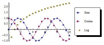
For several years now I am frustrated with how Mathematica plots look. They are sufficient to get an impression of what your data might look like, but they are as far from publication quality as a plot can get. While it is relatively easy to change how a plot looks, the PlotLegends package that comes with Mathematica is not at all nice and can virtually not be customized to give a nice legend. The default look is similar to the following example, which somehow reminds you of excel.

Example of how a default plot legend in Mathematica looks

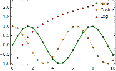
After playing around with Mathematica a bit, I came up with a code that produces the following style of plots:

Example of how I display a plot legend

The code does not do much apart from putting a Grid with plot styles and example icons above the plot. Still I consider the result a major improvement in comparison with the standard Mathematica plot legend.

You can find a copy of my code which also produces the sample plot above at my dropbox.

Creative Commons License
This work is licensed under a Creative Commons Attribution-NonCommercial-ShareAlike 3.0 Unported License.

Tune / Resonance diagram

In Accelerator physics you often need a Tune diagram to display machine tunes. A quick Google search gave me no readily available Mathematica code for drawing one, so I came up with a Mathematica notebook that produces graphics similar to the following diagram:

The Mathematica notebook and package I used to generate the diagram can be found here, a demo Notebook showing the usage of the resonance diagram is included.

To find resonances up to order o I solve the equation
$latex a Q_x +bQ_y=n$
for a list of x and y between –o and o and then plot all those solutions after filtering out solutions for orders higher than desired order. Each solution gets a plot style from a list corresponding to its order.

Feel free to use and modify the notebook, it is, as everything here released under a creative commons license.

Creative Commons License
This work is licensed under a Creative Commons Attribution-NonCommercial-ShareAlike 3.0 Unported License.